 |
| Aussie League BlogSee all entries in this blog |
Excel Attributes Spreadsheet Version 2 (10/02/2009 05:52) |
After making my last blog, I realised that explaining how to create the spreadsheet would not be adequate as it required some effort and too many things could go wrong. To correct this I have improved the spreadsheet so that it only requires the copying and pasting of macros and the spreadsheet setup macro will set up all of the formatting and formulae etc. that the spreadsheet needs. I have also expanded it to cater for 33 players in a squad. The spreadsheet. Please Note: This spreadsheet has been designed in Excel 2003 and my short testing in Excel 2007 shows that it is functional but some of the formulae and formatting are not being set up properly. This may mean that you have to try to set up the formulae manually from my previous blog :o I personally don't use Excel 2007 and get frustrated with the ribbon so may or may not work out the problems. I don't have an internet enabled computer with Excel 97 or 2000 so have not tested the macros in either. Please Note: The process of copying and pasting will not work with Microsoft Internet Explorer. For some reason the copied data is pasted as one continuous row ... take Spinner's advice and upgrade (that is right, you will notice the improvement) to Mozilla Firefox, Google Chrome or Opera ;) I haven't tested this with Opera either but I know that it works with Firefox and Chrome. The spreadsheet is designed to make it easier to distinguish which players have gained attributes since the last copy and paste and show the players' total gains for the season which makes it easier to choose an attribute to train during training or training camps. The completed operational spreadsheet should look like below. If you look where the cursor was on the screenshot, you will notice that I have added a function to highlight the row when a player gains an attribute, the attribute is highlighted and a "tooltip" shows which sort of attribute it was (+1 Heading for Robert Thorkildsen in this case). 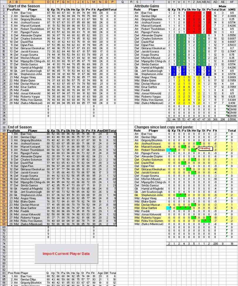 Building the Spreadsheet. Step One. Open Microsoft Excel with a new blank spreadsheet. Select "Tools -> Macros -> Visual Basic Editor" from the menu (or press Alt+F11) which will start the Visual Basic Editor (VBE) that is contained within Excel. Go to "Insert -> Module" on the menu. An empty sheet will appear and this is where you paste the macros from below. Copy the macro below (within the lines) and go back to the Visual Basic Editor and paste it into the module. This is the macro that performs all the day-to day operations of the spreadsheet. When you paste it into the module you will notice that lines that are after an apostrophe (') are in green - these are comments are my attempt to explain what each part is for if you wish to look at the code. Sub ImportPlayerData() 'Paste the copied data Range("A83").Select ActiveSheet.PasteSpecial Format:="Unicode Text", Link:=False, _ DisplayAsIcon:=False 'Delete the unrequired data eg Age, Resting, Training Now columns. Range("O83:P116").Select Selection.Delete Shift:=xlToLeft 'Sort the data into positions and then alphabetical order Range("B84:P116").Select Selection.Sort Key1:=Range("B83"), Order1:=xlAscending, Key2:=Range("C83" _ ), Order2:=xlAscending, Header:=xlNo, OrderCustom:=1, MatchCase:= _ False, Orientation:=xlTopToBottom, DataOption1:=xlSortNormal, DataOption2 _ :=xlSortNormal ' Remove the Q increase from the right of the Q value Dim c As Variant Dim d As Variant Dim remover As Variant For Each c In Range("D84:D116") d = c.Value remover = Val(d) c.Value = remover Next 'Remove the "Inj" from the fitness of injured players (not required when copying from Google Chrome) Dim e As Variant Dim f As Variant Dim remover2 As Variant For Each e In Range("M84:M116") f = e.Value remover = Val(f) e.Value = remover Next 'Start the macro called CalcChanges Call CalcChanges 'Copy the data from Section 3 to Section 2 Range("B84:P116").Select Selection.Copy Range("B40").Select ActiveSheet.Paste End Sub Sub CalcChanges() 'Clear the old comments in Section 5 Range("U40:AD72").Select Selection.ClearComments 'Clear old colour fills Range("S40:AF74").Select Selection.Interior.ColorIndex = xlNone 'Compare the cells from Section 3 to Section 2 to calculate attribute increases 'since last paste and put them into section 5 Range("U40:AD72") = Evaluate("D84:M116-D40:M72") 'Format the cells with attribute gains Dim x1 As Range Dim x2 As Range 'Change the background and add comment for each cell that has an attribute increase For Each a In Range("U40:U72") If a.Value > 0 Then 'Change the fill colour of the row Set x1 = a.Offset(0, -2) Set x2 = a.Offset(0, 11) Range(x1, x2).Select Selection.Interior.ColorIndex = 36 'cream 'Change the cell fill colour and add comment a.Interior.ColorIndex = 8 'cyan a.AddComment a.Comment.Visible = False a.Comment.Text Text:="Quality" End If Next For Each a In Range("V40:V72") If a.Value > 0 Then 'Change the fill colour of the row Set x1 = a.Offset(0, -3) Set x2 = a.Offset(0, 10) Range(x1, x2).Select If Selection.Interior.ColorIndex = xlNone Then Selection.Interior.ColorIndex = 36 'cream a.Interior.ColorIndex = 4 'green a.AddComment a.Comment.Visible = False a.Comment.Text Text:="Keeping" End If Next For Each a In Range("W40:W72") If a.Value > 0 Then 'Change the fill colour of the row Set x1 = a.Offset(0, -4) Set x2 = a.Offset(0, 9) Range(x1, x2).Select If Selection.Interior.ColorIndex = xlNone Then Selection.Interior.ColorIndex = 36 'cream a.Interior.ColorIndex = 4 'green a.AddComment a.Comment.Visible = False a.Comment.Text Text:="Tackling" End If Next For Each a In Range("X40:X72") If a.Value > 0 Then 'Change the fill colour of the row Set x1 = a.Offset(0, -5) Set x2 = a.Offset(0, 8) Range(x1, x2).Select If Selection.Interior.ColorIndex = xlNone Then Selection.Interior.ColorIndex = 36 'cream a.Interior.ColorIndex = 4 'green a.AddComment a.Comment.Visible = False a.Comment.Text Text:="Passing" End If Next For Each a In Range("Y40:Y72") If a.Value > 0 Then 'Change the fill colour of the row Set x1 = a.Offset(0, -6) Set x2 = a.Offset(0, 7) Range(x1, x2).Select If Selection.Interior.ColorIndex = xlNone Then Selection.Interior.ColorIndex = 36 'cream a.Interior.ColorIndex = 4 'green a.AddComment a.Comment.Visible = False a.Comment.Text Text:="Shooting" End If Next For Each a In Range("Z40:Z72") If a.Value > 0 Then 'Change the fill colour of the row Set x1 = a.Offset(0, -7) Set x2 = a.Offset(0, 6) Range(x1, x2).Select If Selection.Interior.ColorIndex = xlNone Then Selection.Interior.ColorIndex = 36 'cream a.Interior.ColorIndex = 4 'green a.AddComment a.Comment.Visible = False a.Comment.Text Text:="Heading" End If Next For Each a In Range("AA40:AA72") If a.Value > 0 Then 'Change the fill colour of the row Set x1 = a.Offset(0, -8) Set x2 = a.Offset(0, 5) Range(x1, x2).Select If Selection.Interior.ColorIndex = xlNone Then Selection.Interior.ColorIndex = 36 'cream a.Interior.ColorIndex = 4 'green a.AddComment a.Comment.Visible = False a.Comment.Text Text:="Speed" End If Next For Each a In Range("AB40:AB72") If a.Value > 0 Then 'Change the fill colour of the row Set x1 = a.Offset(0, -9) Set x2 = a.Offset(0, 4) Range(x1, x2).Select If Selection.Interior.ColorIndex = xlNone Then Selection.Interior.ColorIndex = 36 'cream a.Interior.ColorIndex = 4 'green a.AddComment a.Comment.Visible = False a.Comment.Text Text:="Stamina" End If Next For Each a In Range("AC40:AC72") If a.Value > 0 Then 'Change the fill colour of the row Set x1 = a.Offset(0, -10) Set x2 = a.Offset(0, 3) Range(x1, x2).Select If Selection.Interior.ColorIndex = xlNone Then Selection.Interior.ColorIndex = 36 'cream a.Interior.ColorIndex = 4 'green a.AddComment a.Comment.Visible = False a.Comment.Text Text:="Perception" End If Next 'Change the size of comments (code adapted from Ivan Moala's code) and the font in comments Dim AllComments As Range Dim ComCell As Range On Error Resume Next Set AllComments = Range("U40:AD72").SpecialCells(xlCellTypeComments) If AllComments Is Nothing And Not All Then GoTo GetOut For Each ComCell In AllComments With ComCell.Comment .Shape.Height = .Shape.Height * 0.27 .Shape.Width = .Shape.Width * 0.55 .Shape.TextFrame.Characters.Font.ColorIndex = 3 .Shape.TextFrame.Characters.Font.Name = "arial" .Shape.TextFrame.Characters.Font.Size = 10 .Shape.TextFrame.Characters.Font.Bold = False End With Next ComCell GetOut: End Sub Sub ColourChanger() 'Change the background colour according to the main stats of different positions in Section 4 Dim a As Variant Range("S3").Activate For Each a In Range("S3:S35") If a.Value = "Att" Then ActiveCell.Offset(0, 6).Select Selection.Interior.ColorIndex = 3 'red ActiveCell.Offset(0, 1).Select Selection.Interior.ColorIndex = 3 'red ActiveCell.Offset(0, 1).Select Selection.Interior.ColorIndex = 3 'red ActiveCell.Offset(0, 2).Select Selection.Interior.ColorIndex = 3 'red ActiveCell.Offset(1, -10).Select ElseIf a.Value = "Def" Then ActiveCell.Offset(0, 4).Select Selection.Interior.ColorIndex = 50 'green Selection.Font.ColorIndex = 6 'yellow ActiveCell.Offset(0, 1).Select Selection.Interior.ColorIndex = 50 'green Selection.Font.ColorIndex = 6 'yellow ActiveCell.Offset(0, 3).Select Selection.Interior.ColorIndex = 50 'green Selection.Font.ColorIndex = 6 'yellow ActiveCell.Offset(0, 1).Select Selection.Interior.ColorIndex = 50 'green Selection.Font.ColorIndex = 6 'yellow ActiveCell.Offset(1, -9).Select ElseIf a.Value = "Gk" Then ActiveCell.Offset(0, 3).Select Selection.Interior.ColorIndex = 5 'blue Selection.Font.ColorIndex = 6 'yellow ActiveCell.Offset(0, 2).Select Selection.Interior.ColorIndex = 5 'blue Selection.Font.ColorIndex = 6 'yellow ActiveCell.Offset(0, 3).Select Selection.Interior.ColorIndex = 5 'blue Selection.Font.ColorIndex = 6 'yellow ActiveCell.Offset(0, 2).Select Selection.Interior.ColorIndex = 5 'blue Selection.Font.ColorIndex = 6 'yellow ActiveCell.Offset(1, -10).Select ElseIf a.Value = "Mid" Then ActiveCell.Offset(0, 4).Select Selection.Interior.ColorIndex = 6 'yellow ActiveCell.Offset(0, 1).Select Selection.Interior.ColorIndex = 6 'yellow ActiveCell.Offset(0, 1).Select Selection.Interior.ColorIndex = 6 'yellow ActiveCell.Offset(0, 2).Select Selection.Interior.ColorIndex = 6 'yellow ActiveCell.Offset(1, -8).Select End If Next End Sub Sub MSFormula() 'Create the fomula to add up the main stats in Section 4 Dim a As Variant Range("S3").Activate For Each a In Range("S3:S35") If a.Value = "Att" Then ActiveCell.Offset(0, 12).Select ActiveCell.FormulaR1C1 = "=RC[-6]+RC[-5]+RC[-4]+RC[-2]" ActiveCell.Offset(1, -12).Select ElseIf a.Value = "Def" Then ActiveCell.Offset(0, 12).Select ActiveCell.FormulaR1C1 = "=RC[-8]+RC[-7]+RC[-4]+RC[-3]" ActiveCell.Offset(1, -12).Select ElseIf a.Value = "Gk" Then ActiveCell.Offset(0, 12).Select ActiveCell.FormulaR1C1 = "=RC[-9]+RC[-7]+RC[-4]+RC[-2]" ActiveCell.Offset(1, -12).Select ElseIf a.Value = "Mid" Then ActiveCell.Offset(0, 12).Select ActiveCell.FormulaR1C1 = "=RC[-8]+RC[-7]+RC[-6]+RC[-4]" ActiveCell.Offset(1, -12).Select End If Next End Sub Second Set of Macros Insert another module in the VBE ("Insert -> Module") and copy the next macro into the new module that is called Module 2. This second set of macros is all to do with setting up the spreadsheet (DO NOT run it yet!). It will put the appropriate formulae where they are required, put the headings where they are required, and do all the relevant formatting (eg colouring the boxes in Section 4 etc.). These macros will be only used once but you can leave them in the workbook just in case you wish to start the spreadsheet again. Sub Setup_Spreadsheet() 'Rename Sheet1 to Attributes Worksheets(1).Name = "Attributes" Worksheets("Attributes").Activate 'Paste the data from ML into the spreadsheet Call ImportPlayerData 'Paste the Square of data around the page Range("A83:P116").Select Selection.Copy Range("A39").Select ActiveSheet.Paste Range("R39").Select ActiveSheet.Paste Range("A2").Select ActiveSheet.Paste Range("R2").Select ActiveSheet.Paste Worksheets("Attributes").Columns("A:AG").AutoFit Range("Q1:R73").ClearContents 'Start the setup of formulae through the SetupFormulae macro :) Call SetupFormulae 'Setup the Main Stat Formulae in column AE Call MSFormula 'Start the Colour Changer macro for Section 4 Call ColourChanger 'Start the extra formatting code Call Formatting 'Start the code for creating the Insert/Delete Player dialogs NB Unused now ' Call CreateDialogs End Sub Sub SetupFormulae() 'Setup Section 4 Range("U3").Select ActiveCell.FormulaR1C1 = "=R[37]C[-17]-RC[-17]" Selection.AutoFill Destination:=Range("U3:U35"), Type:=xlFillDefault Range("U3:U35").Select Selection.AutoFill Destination:=Range("U3:AD35"), Type:=xlFillDefault Range("U36").Select ActiveCell.FormulaR1C1 = "=SUM(R[-33]C:R[-1]C)" Selection.AutoFill Destination:=Range("U36:AF36"), Type:=xlFillDefault Range("AD2").Select ActiveCell.FormulaR1C1 = "Total" Range("AE1").Select ActiveCell.FormulaR1C1 = "Main" Range("AE2").Select ActiveCell.FormulaR1C1 = "Stat" Range("AF2").Select ActiveCell.FormulaR1C1 = "%MS" Range("AG2:AG72").ClearContents Range("AD3").Select ActiveCell.FormulaR1C1 = "=SUM(RC[-1])" Selection.AutoFill Destination:=Range("AD3:AD35"), Type:=xlFillDefault Range("AF3").Select ActiveCell.FormulaR1C1 = "=RC[-1]/RC[-2]" Selection.AutoFill Destination:=Range("AF3:AF36"), Type:=xlFillDefault 'Put border around formulae Range("U36:AF36").Select With Selection.Borders(xlEdgeTop) .LineStyle = xlContinuous .Weight = xlThin .ColorIndex = xlAutomatic End With With Selection.Borders(xlEdgeBottom) .LineStyle = xlDouble .Weight = xlThick .ColorIndex = xlAutomatic End With 'Setup Section 5 Range("U40:AF69").ClearContents Range("AE39:AF39").ClearContents Range("AF39").Select ActiveCell.FormulaR1C1 = "Total" Range("AF40").Select ActiveCell.FormulaR1C1 = "=SUM(RC[-10]:RC[-3])" Selection.AutoFill Destination:=Range("AF40:AF72"), Type:=xlFillDefault Range("U74").Select ActiveCell.FormulaR1C1 = "=SUM(R[-34]C:R[-1]C)" Selection.AutoFill Destination:=Range("U74:AF74"), Type:=xlFillDefault 'Put border around formulae Range("U74:AF74").Select With Selection.Borders(xlEdgeTop) .LineStyle = xlContinuous .Weight = xlThin .ColorIndex = xlAutomatic End With With Selection.Borders(xlEdgeBottom) .LineStyle = xlDouble .Weight = xlThick .ColorIndex = xlAutomatic End With 'Centre the alignment on all tables Range("U3:AF36").HorizontalAlignment = xlCenter Range("D3:P35").HorizontalAlignment = xlCenter Range("D40:P72").HorizontalAlignment = xlCenter Range("U40:AF74").HorizontalAlignment = xlCenter Range("D84:P116").HorizontalAlignment = xlCenter 'Bolden and centre the top line of each section Range("S39:AF39").Select Selection.Font.Bold = True Selection.HorizontalAlignment = xlCenter Range("S1:AF2").Select Selection.Font.Bold = True Selection.HorizontalAlignment = xlCenter Range("A2:P2").Select Selection.Font.Bold = True Selection.HorizontalAlignment = xlCenter Range("A39:P39").Select Selection.Font.Bold = True Selection.HorizontalAlignment = xlCenter End Sub Sub Formatting() 'Autofit column widths Worksheets("Attributes").Columns("A:AG").AutoFit 'Add titles to each Section. Range("A1").Select ActiveCell.FormulaR1C1 = "Start of the Season" Selection.Font.Size = 14 Selection.Font.Bold = True Selection.HorizontalAlignment = xlLeft Range("S1").Select ActiveCell.FormulaR1C1 = "Attribute Gains" Selection.Font.Size = 14 Selection.Font.Bold = True Selection.HorizontalAlignment = xlLeft Range("A38").Select ActiveCell.FormulaR1C1 = "End of Season" Selection.Font.Size = 14 Selection.Font.Bold = True Selection.HorizontalAlignment = xlLeft Range("S38").Select ActiveCell.FormulaR1C1 = "Changes since last copy and paste:" Selection.Font.Size = 14 Selection.Font.Bold = True Selection.HorizontalAlignment = xlLeft 'Autofit row heights to allow for the new titles Worksheets("Attributes").Rows("1:116").AutoFit 'Create the Command Button Worksheets(1).OLEObjects.Add "Forms.CommandButton.1", Left:=110, Top:=950, Width:=250, _ Height:=80 End Sub Third Macro Insert another module in the VBE ("Insert -> Module") and copy the next macro into the new module that is called Module 3. This macro formats the button on the spreadsheet so that it is nice and pretty :). This last macro will have to be run separately after the whole spreadsheet is set up Sub FormatButton() With Worksheets(1).CommandButton1 .Caption = "Import Current Player Data" .Font.Size = 14 .Font.Bold = True .ForeColor = &HFF& .MousePointer = 10 End With End Sub Save the Excel workbook with whatever name you choose - I use Attributes Season 45 etc. Please continue to the next page to see how to finalise the set-up in Step Two. |
| Share on Facebook |
| This blogger owns the team Srennug Lanesra. (TEAM:7937) |
|
You are currently not logged into ManagerLeague If you wish to log in, click here. If you wish to sign up and join us, click here. |
|
| Rational wrote: 15:39 15/02 2009 |
|

| Zz00352679 wrote: 12:44 20/11 2010 |
|

| Zz00559205 wrote: 15:47 30/06 2011 |
|

| Post a comment |
|
| © 2003-2007 Fifth Season AS, Oslo, Norway. Privacy Policy. Rules and Code of Conduct. Sitemap. Responsible Editor for ManagerLeague is Christian Lassem. |